Several years ago, some of my bicycling friends told me that they just never “got” calculus. I took this as a personal challenge. I told them that I could explain the basics of differential calculus to them in 5 minutes.

How did I do that? By relating it to something they already understood at an intuitive level, something they used on all of their bike rides – their bike computers.

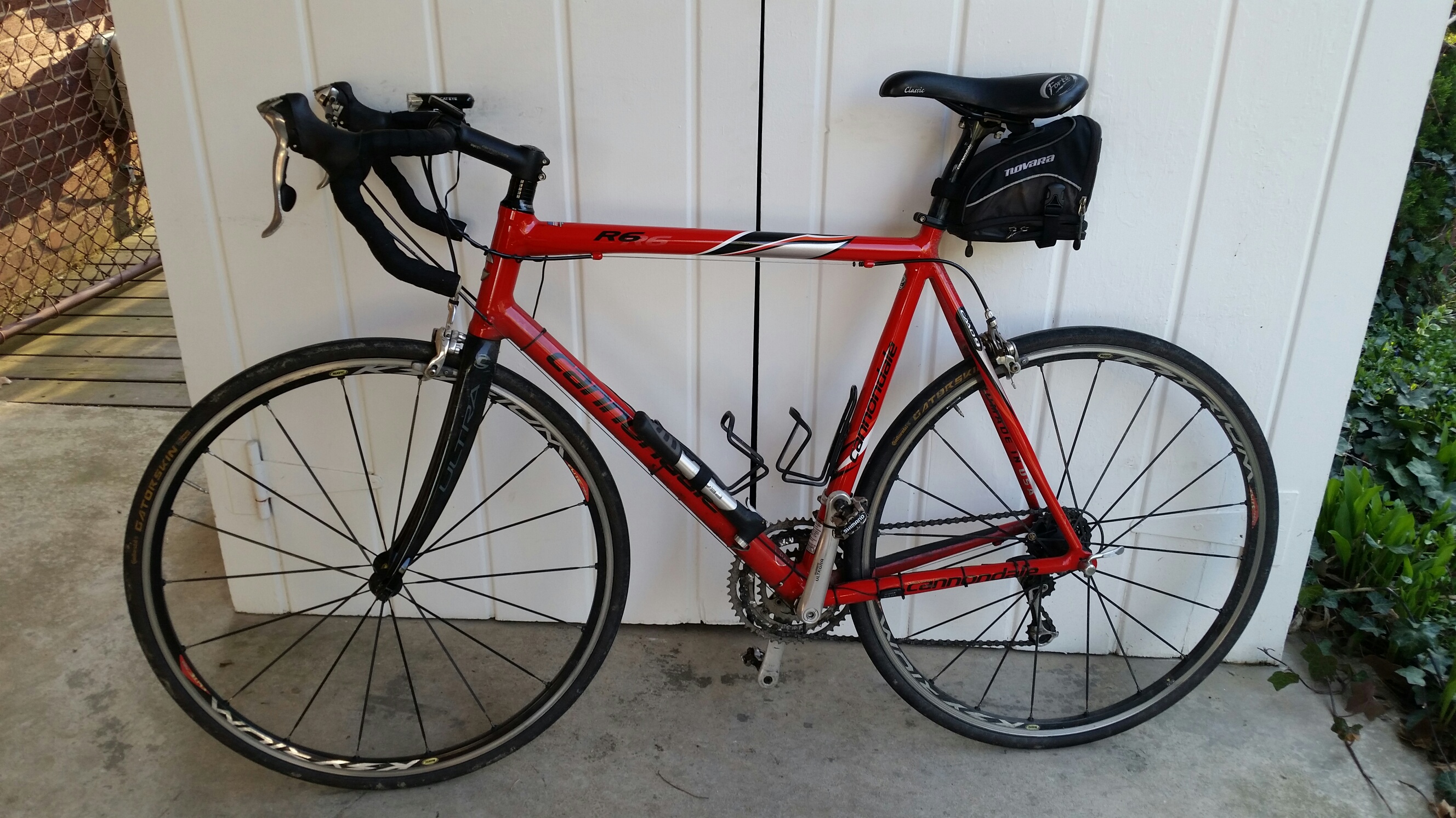
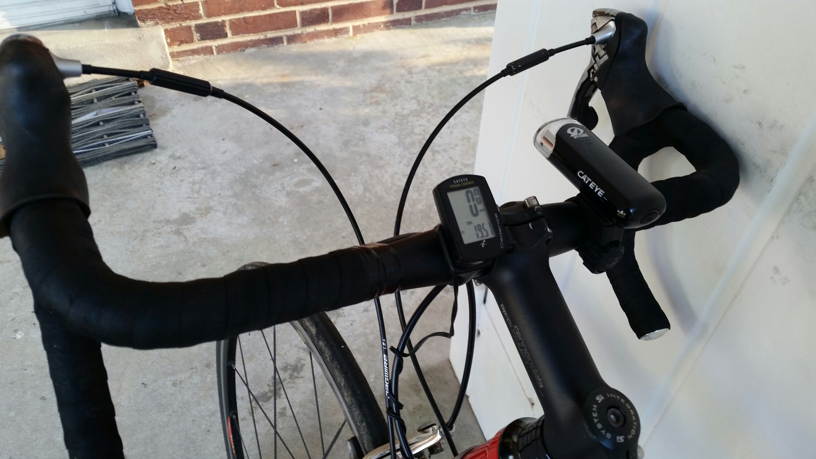
The main part of a bike computer, which includes the processor and the display, mounts on your handlebars where you can see it.

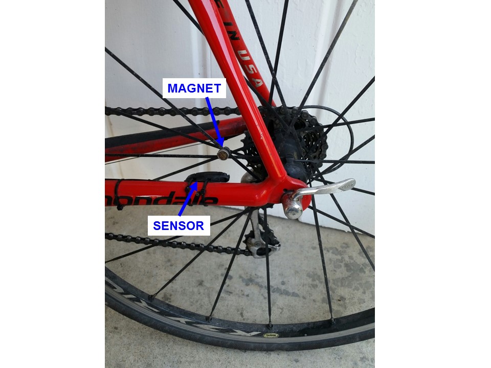
It is connected to a magnetic sensor that mounts on the frame near one of the wheels. A magnet is mounted on one of the spokes. Each time the magnetic passes the sensor, the sensor sends a “tick” to the processor, telling it that the wheel has just completed one revolution. Each tick tells the computer that the bike has just moved a distance corresponding to the circumference of your wheel.

While setting up the computer before riding, one of the key steps is to program in your wheel’s circumference. This can be measured by stretching a tape measure out on the floor, rolling your bike along it, and determining the length corresponding to a full revolution of the wheel. (I usually use the valve stem as a reference point.) Wheels on typical adult sized bikes will have a circumference of around 6 ½ feet, or a bit over 2 meters.

OK, so now your computer is counting ticks and adding the wheel circumference for each tick to tell you the distance you have travelled. That explains the odometer function of your computer, which is one piece of the differential calculus puzzle.

The computer also has a timer in it, i.e. a clock. While counting ticks and adding up distances, it also counts how much time elapses between ticks. Speed is simply distance travelled divided by time elapsed, as indicated by the units, e.g. miles per hour (mph), meters per second, furlongs per fortnight, light-years per…year, etc.

For the sake of illustration, let’s say your computer records your distance travelled once per hour. If after one hour, you have travelled 15 miles, then your average speed over that one hour period is:

(15 miles) / (1 hour) = 15 miles per hour (mph)

But I imagine that you would prefer to wait a bit less than one hour to find out your speed.

Let’s say your computer records your distance travelled every 15 minutes, or every ¼ hour. If in 15 minutes you have travelled 5 miles, then your average speed over that 15 minute period is:

(5 miles) / (1/4 hour) = 20 miles per hour

At 20 mph, you’re moving along at a pretty good clip. But again, 15 minutes is awhile to wait to find out your speed.

Let’s say your computer records your distance travelled every 1 minute, or every 1/60 hour. If in 1 minute you have travelled 1/2 mile, then your average speed over that 1 minute period is:

(1/2 mile) / (1/60 hour) = 30 miles per hour

Now you’re really cruising. But a full minute is still a pretty long time to wait.

Now let’s say your computer records your distance travelled every 1 second, which equals 1/60 of a minute, which equals 1/3600 of an hour. This is much more realistic, and it is close the update rate most bike computers use. If in 1 second you have travelled 52.8 feet, which equals 1/100 of a mile (1 mile = 5280 feet), then your average speed over that 1 second period is:

(1/100 mile) / (1/3600 hour) = 36 miles per hour

At this speed, you are likely either 1) training for the Tour de France, or 2) going down a pretty steep hill, yelling “WOO-HOO!!!” (Possibly both; they are not mutually exclusive options.)

“That’s all well and good,” you’re saying, “but what does all this have to do with differential calculus?”

Everything.

As Frank Zappa used to say, this is “the crux of the biscuit.”

Differential calculus is all about finding the instantaneous rate of change of one quantity with respect to another. In this example, we are looking at the change of distance with respect to time, which is the very definition of speed. We have been looking at the average rate of change over shorter and shorter intervals of time.

Note that is the changes in distance and time that are important here, NOT absolute distance and time. My bike computer does not know nor care whether I am 10, 20, or 100 miles from my house. All it cares about is the change in distance, or the difference in distance (hence the term “differential calculus”). The change in a quantity is expressed by the Greek letter Δ (upper case “Delta”), and it can be expressed as a subtraction of the distance d₁ at the beginning of the interval from the distance d₂ at the end of the interval:

Δd = d₂ – d₁

Likewise, my computer does not know nor care whether it is 6:00 AM, noon, or midnight. All it cares about is the difference in time over the interval measured. This can be similarly expressed as a subtraction of the time t₁ at the beginning of the interval from the time t₂ at the end of the interval:

Δt = t₂ – t₁

Average speed v_av over a time interval is simply the change in distance divided by the change in time:

v_av = Δd / Δt = (d₂ – d₁) / (t₂ – t₁)

To get the true instantaneous speed v_inst, we would have to shorten the interval of time Δt to, ideally, 0. In mathematical parlance, we would “take the limit as Δt approaches 0”:

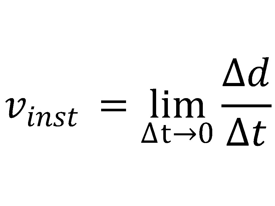
In real life, this is rather difficult to do. But we can approximate it by making the time interval small enough that it gives a good approximation to the instantaneous speed.

In this example, taking a sample approximately once per second works pretty darned well. I don’t know too many cyclists who can significantly change their speed over a 1 second period. It’s still gives you an average speed, but it’s close enough to an instantaneous speed for most practical purposes.

And what are the mathematical operations at the heart of all of this? Subtraction and division, i.e. basic arithmetic., Q.E.D. This it is, and nothing more.

For the record, the above explanation worked; my friends came away from it with an intuitive grasp of differential calculus that they did not previously have. Now that I think about it, that very interaction probably planted one of the earliest seeds that led to my desire to make math more understandable and less horrifying to people.

Integral Calculus is essentially the reverse of differential calculus.  Take a look at that page next.